Innovations in BIM-based Localization

In the classic SLAM context, the process involves simultaneous mapping and localization (SLAM), meaning that the map is built incrementally while the robot's location is estimated.

However, in the construction context, the map only needs to be constructed once and can support long-term operations. Moreover, BIM is becoming more prevalent compared to CAD. Against this backdrop, the following three studies focus on BIM-based localization, semantic consistency, and geometric consistency.

Towards BIM-based Localization

H. Yin, J. M. Liew, W. L. Lee, M. H. Ang, Ker-Wei Yeoh, and Justin, “Towards BIM-based robot localization: a real-world case study,” presented at the 39th International Symposium on Automation and Robotics in Construction, Jul. 2022. doi: 10.22260/ISARC2022/0012.

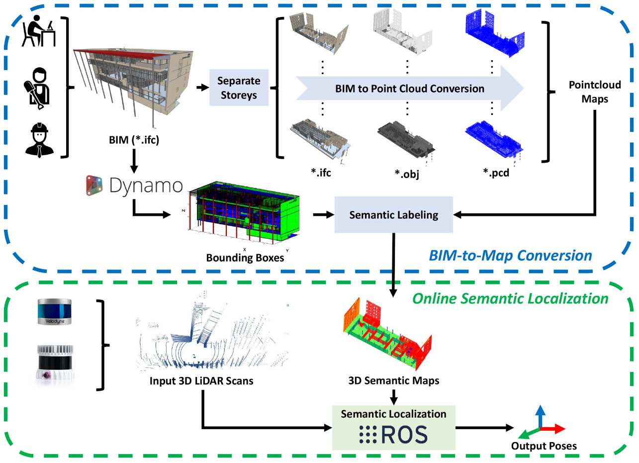
This work leverages a workflow that localizes robots in BIM-generated maps, freeing them from the computational complexity and global inconsistency of online SLAM.

Mapping

The authors propose a three-step pipeline for each individual floor:

Localization

A point-to-plane ICP-based pose estimation algorithm is used:

$$(\mathrm{R},\mathrm{t})=\arg \underset{(\mathrm{R},\mathrm{t})}{min}(\sum _{k=1}^K||({\mathrm{R}\mathrm{p}}_k+{\mathrm{t}-\mathrm{q}}_k)\cdot {\mathrm{n}}_k|{|}_2)$$

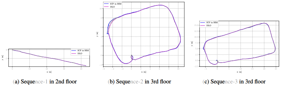
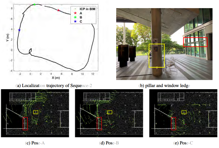
In the NUS dataset, localization achieves translation errors below 0.2m and rotation errors below 2° compared to DLO. However, deviations between as-planned and as-built conditions can lead to sudden drift.

Why not DLO ?

Direct LiDAR Odometry (DLO) achieves even higher accuracy than other LiDAR SLAM systems, to the point where the authors use it as a proxy for ground truth in their experiments. So why not rely entirely on DLO?

Despite its superior accuracy, DLO still suffers from global inconsistency due to its scan-to-scan matching approach. More importantly, DLO cannot leverage the semantic information contained in BIM models.

Towards Semantic Consistency

H. Yin, Z. Lin, and J. K. W. Yeoh, “Semantic localization on BIM-generated maps using a 3D LiDAR sensor,” Automation in Construction, vol. 146, p. 104641, Feb. 2023, doi: 10.1016/j.autcon.2022.104641.

This work introduces Semantic ICP to improve localization accuracy in structured environments, which guides LiDAR-based localization to both geometric and semantic consist.

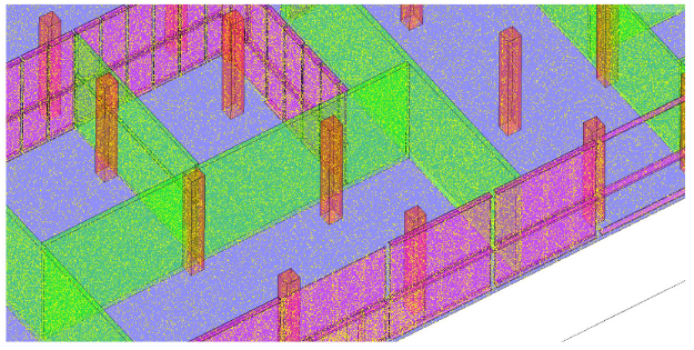
Mapping

Each semantic object in BIM is represented by an axis-aligned bounding box which is parameterized by 2 points ${\mathrm{d}}_{\mathrm{m}\mathrm{i}\mathrm{n}}=[{\mathrm{x}}_{\mathrm{m}\mathrm{i}\mathrm{n}},{\mathrm{y}}_{\mathrm{m}\mathrm{i}\mathrm{n}},{\mathrm{z}}_{\mathrm{m}\mathrm{i}\mathrm{n}}{]}^{\mathrm{T}}$ and ${\mathrm{d}}_{\mathrm{m}\mathrm{a}\mathrm{x}}=[{\mathrm{x}}_{\mathrm{m}\mathrm{a}\mathrm{x}},{\mathrm{y}}_{\mathrm{m}\mathrm{a}\mathrm{x}},{\mathrm{z}}_{\mathrm{m}\mathrm{a}\mathrm{x}}{]}^{\mathrm{T}}$. A point is labeled if it lies within a box, assigning it the corresponding semantic class. While this approach may introduce minor inaccuracies - such as oversized boxes for non-axis-aligned walls or ambiguous labels for boundary points - the impact on overall localization performance is negligible.

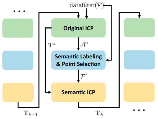
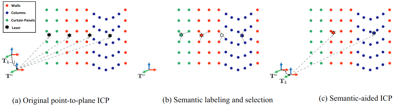
Localization

With the guidance of coarse-to-fine, there are three steps to achieving the refined result. First, iterate by standard ICP to get a coarse result. Then, based on that result, the input points are labeled with those boxes. Finally, based on the label, a semantic ICP is applied to refined registration.

$$\mathbf{T}=\arg \underset{\mathbf{T}}{min}(\sum _{(i,j)}w({\mathbf{x}}_i^r,{\mathbf{x}}_j^t)\cdot r({\mathbf{x}}_i^r,{\mathbf{x}}_j^t))$$

Which

$$w_c=\{\begin{array}{ll}\mu ,& \text{same label}\\ 1-\mu ,& \text{otherwise}\end{array}$$

In Huan's practice, $\mu$ is chosen to be $0.8$ while $\delta$ is chosen to be $0.05(\mathrm{m})$.

$$w_p=\{\begin{array}{ll}1,& e(·)<\delta \\ \delta /e(·),& e(·)\ge \delta \end{array}$$

In the experiment, a 2D offline SOTA SLAM Cartographer is chosen as a proxy for ground truth. Compared to standard ICP, the semantic filter improved the accuracy, while the gap between as-designed and as-built was still unsolved. The conversion from BIM to a semantic map may not be that accurate, which may reduce the robustness. The init guess of ${\mathrm{T}}_k$ relies on ${\mathrm{T}}_{k-1}$, a significant error in ${\mathrm{T}}_k$ would lead to catastrophic sequence.

Towards Geometric Consistency

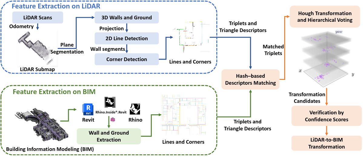
Z. Qiao et al., “Speak the Same Language: Global LiDAR Registration on BIM Using Pose Hough Transform,” IEEE Transactions on Automation Science and Engineering, pp. 1–1, 2025, doi: 10.1109/TASE.2025.3549176.

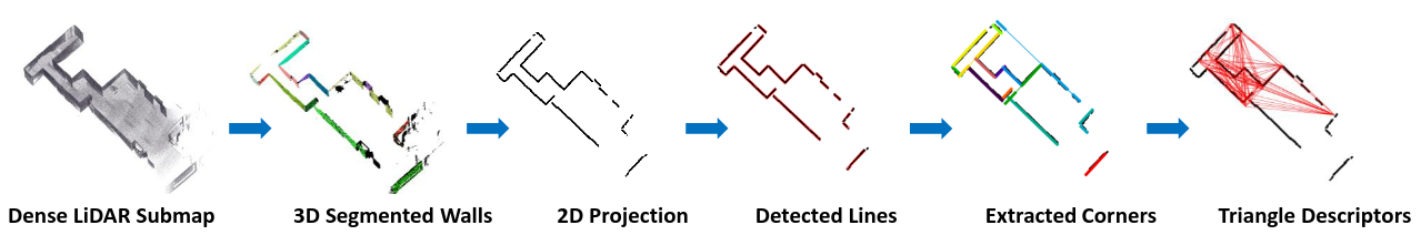
Submap is composed by a sequence of pointcloud inputs

$$\mathcal{S}=\mathrm{\Gamma }(\bigcup _{k=1}^n{\mathbf{T}}_k{\mathcal{P}}_k,r_v)$$

$\mathrm{\Gamma }(\mathcal{S},r)$ is voxelization downsampling function，$r_v=0.8\mathrm{m}$ represents the voxel size，$n$ is the minimum number of scans required such that traversed distance exceeds $d_s$ meters.

Every voxel is parameterized by Gaussian distribution

$$\overline{\mathbf{p}}=\frac{1}{N}\sum _{i=1}^N{\mathbf{p}}_i,\mathrm{\Sigma }=\frac{1}{N}\sum _{i=1}^N({\mathbf{p}}_i-\overline{\mathbf{p}})({\mathbf{p}}_i-\overline{\mathbf{p}}{)}^T$$

To determine whether the points in a voxel belong to a plane, we analyze the eigenvalues of the covariance matrix $\mathrm{\Sigma }$. The first eigenvector (associated with the largest eigenvalue) points towards the greatest variance, while the second and third eigenvectors correspond to the next greatest variances. Hence, ${\lambda }_2/{\lambda }_3$ will be compared with the threshold ${\sigma }_{\lambda }=10$ to determine whether the voxel belongs to a planar. If the ratio does not meet the threshold, the voxel is further subdivided into four sub-voxels (? Is it only divided in the horizontal direction? No corresponding code has been found yet), and the plane identification process is repeated until each sub-voxel contains fewer than four points.

After this, those voxels with similar normal and similar point-to-plane distances will merge into the same planar. Then wall points are projected onto the ground plane with a pixel scale of $s_I=60\mathrm{p}\mathrm{x}/\mathrm{m}$, with a Hough Transform-based line segment detector applied to extract the wall. Short 2D line segments (length under $L_{\text{min}}=30\mathrm{p}\mathrm{x}$) are discarded, while the remaining segments are merged based on endpoint proximity and directional similarity, then refitted to the original points for geometric accuracy. The refitted lines are extended a predefined distance to intersect and form corners, which are further refined using Non-Maximum Suppression (NMS) to avoid clustering.

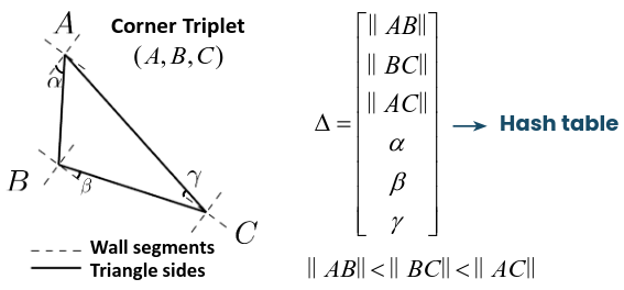
The triangle descriptor $\mathrm{\Delta }=[||AB||,||BC||,||AC||,\alpha ,\beta ,\gamma ]$ are quantized based on side length resolution $r_s=0.5\mathrm{m}$ and angle resolution $r_a=3.0\mathrm{d}\mathrm{e}\mathrm{g}$. Although it leads to a high outlier ratio, the likelihood of candidates is also high. For every corner triplets $(A,B,C)$ within the range $L_{\mathrm{m}\mathrm{a}\mathrm{x}}=30.0\mathrm{m}\text{ or }40.0\mathrm{m}$, a triangle descriptor will be calculated and stored in the hash table. When querying, it nearly costs a constant time.

Based on the resolution of $0.15\mathrm{m}$ for translation and $1.0\mathrm{d}\mathrm{e}\mathrm{g}$ for rotation, an accumulated tensor is formed for transforming matching to $se(2)$ parameter space. First, every match will contribute to some elements in that accumulated tensor. Then the highest $L=10000$ elements will merge their neighborhoods' value. For the highest $K=5000$ elements, non-maximum depression is applied to filter out $K^{\prime }$ elements. Finally, for the rest of $J=1500$ elements, confidence score will calculated for them one by one.

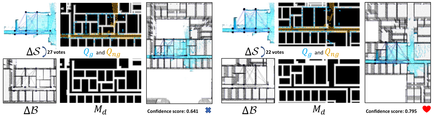
To determine the optimal transformation aligning a LiDAR submap with a BIM model, an occupancy-aware confidence score is proposed. The BIM wall point cloud ${\mathcal{P}}_B$​ is rasterized into a 2D grid $\mathcal{M}$ with resolution $s_r$​, where occupied cells are set to 1 and free cells to 0: $\mathcal{M}=\varphi ({\mathcal{P}}_B,s_r)$. To account for as-built deviations, $\mathcal{M}$ is dilated using a kernel of size $k_d$​, producing a score field ${\mathcal{M}}_d$​ where cell values decrease linearly with distance to the nearest occupied cell. The score evaluates alignment using two components: an award score sasa​ and a penalty score spsp​. The award score rewards matches between non-ground submap points $Q_{ng}$ and BIM walls:

$$s_a=\sum _{q\in Q_{ng}}{\mathcal{M}}_d(\varphi (q,s_r))$$

The penalty score penalizes ground submap points $Q_g$ overlapping with BIM walls:

$$s_p=\sum _{q\in Q_g}{\mathcal{M}}_d(\varphi (q,s_r))$$

The final confidence score combines these components

$$s=\frac{s_a-\lambda \cdot s_p}{|Q_{ng}|}$$

where $\lambda$ balances their contributions, and normalization by $|Q_{ng}$ ensures robustness to submap size. This score avoids biases from unmatched free spaces or real-world objects not in the BIM, providing a reliable measure of alignment quality.

Problems Unsolved

The authors use a clever confidence calculation method to avoid the difference between as-designed and as-built make some effects. It is an implicit way to express the gaps. Do we need to express it explicitly? Can we find an explicit expression for such gaps?

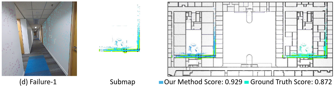
The second problem is lidar would degenerate in long corridor cases, which leads to inconsistency and failure estimation. Do we need to expand the size of the submap to avoid it? Can we use a topologic graph to avoid it explicitly? Or can we fuse more information from other sensors like cameras or radar?