ELEC 5650 - Kalman Filter

"We have decided to call the entire field of control and communication theory, whether in the machine or in the animal, by the name Cybernetics, which we form from the Greek ... for steersman."

 -- by Norbert Wiener

This is the lecture notes for "ELEC 5650: Networked Sensing, Estimation and Control" in the 2024-25 Spring semester, delivered by Prof. Ling Shi at HKUST. In this session, we will deviate Kalman Filter from three different perspectives: Geometric, Probabilistic, and Optimization approaches. Each perspective provides unique insights into understanding and implementing the Kalman Filter algorithm.

1. Mathematic Tools
2. Estimation Theory
3. Kalman Filter <--
4. Linear Quadratic Regulator

Takeaway Notes

Consider an LTI system with initial conditions ${\hat{x}}_{0|0}$ and ${\hat{P}}_{0|0}$

$$\begin{array}{rlr}{x}_{k+1}& =A{x}_k+B{u}_k+{\omega }_k,& {\omega }_k\sim \mathcal{N}(0,Q)\\ y_k& =C{x}_k+{\nu }_k,& {\nu }_k\sim \mathcal{N}(0,R)\end{array}$$

Find the estimation of $x_k$ given $\{u_0,u_1\cdots ,u_k\}$ and $\{y_0,y_1\cdots ,y_k\}$.

Assumptions

1. $(A,B)$ is controllable and $(A,C)$ is observable
2. $Q⪰0,R⪰0,P_0⪰0$
3. ${\omega }_k$, ${\nu }_k$ and ${\hat{x}}_0$ are mutually uncorelated
4. The future state of the system is conditionally independent of the past states given the current state

Time Update

$$\begin{array}{rl}{\hat{x}}_{k|k-1}& =A{\hat{x}}_{k-1|k-1}+B{u}_k\\ {\hat{P}}_{k|k-1}& =A{\hat{P}}_{k-1|k-1}{A}^T+Q\end{array}$$

Measurement Update

$$\begin{array}{rl}{K}_k& ={\hat{P}}_{k|k-1}{C}^T(C{\hat{P}}_{k|k-1}{C}^T+R{)}^{-1}\\ {\hat{x}}_{k|k}& ={\hat{x}}_{k|k-1}+K_k(y_k-C{\hat{x}}_{k|k-1})\\ {\hat{P}}_{k|k}& ={\hat{P}}_{k|k-1}-K_{k}C{\hat{P}}_{k|k-1}=({\hat{P}}_{k|k-1}^{-1}+C^T{R}^{-1}C{)}^{-1}\end{array}$$

Geometric Perspective (LMMSE Estimation)

The Geometric perspective views Kalman Filter as a Linear Minimum Mean Square Error (LMMSE) estimator, which is rooted in orthogonal projection theory in Hilbert space. The key insight is that the Kalman Filter's innovation term $e_k$ is orthogonal to all past observations ${\mathcal{Y}}_{k-1}$, ensuring the new information being incorporated is statistically independent of previous measurements, thus maintaining the estimator's optimality.

Time Update

$$\begin{array}{rl}{\hat{x}}_{k|k-1}& ={\text{proj}}_{{\mathcal{Y}}_{k-1}}(x_k)\\ & ={\text{proj}}_{{\mathcal{Y}}_{k-1}}(A{x}_{k-1}+B{u}_k+{\omega }_k)\\ & =A\cdot {\text{proj}}_{{\mathcal{Y}}_{k-1}}(x_{k-1})+B\cdot {\text{proj}}_{{\mathcal{Y}}_{k-1}}(u_k)+{\text{proj}}_{{\mathcal{Y}}_{k-1}}({\omega }_k)\\ & =A{\hat{x}}_{k-1|k-1}+B{u}_k\\ \\ {\tilde{x}}_{k|k-1}& =x_k-{\hat{x}}_{k|k-1}\\ \\ {\hat{P}}_{k|k-1}& =\mathbb{E}[{\tilde{x}}_{k|k-1}{\tilde{x}}_{k|k-1}^T]\\ & =\mathbb{E}[(x_k-{\hat{x}}_{k|k-1})(x_k-{\hat{x}}_{k|k-1}{)}^T]\\ & =\mathbb{E}[(A{\tilde{x}}_{k-1|k-1}+{\omega }_k)(A{\tilde{x}}_{k-1|k-1}+{\omega }_k{)}^T]\\ & =A\mathbb{E}[{\tilde{x}}_{k-1|k-1}{\tilde{x}}_{k-1|k-1}^T]A^T+2A\mathbb{E}[{\tilde{x}}_{k-1|k-1}{\omega }_k^T]+\mathbb{E}[{\omega }_k{\omega }_k^T]\\ & =A{\hat{P}}_{k-1|k-1}{A}^T+Q\end{array}$$

Measurement Update

$$\begin{array}{rl}{e}_k& =y_k-{\hat{y}}_{k|k-1}\\ & =y_k-{\text{proj}}_{{\mathcal{Y}}_{k-1}}(y_k)\\ & =y_k-{\text{proj}}_{{\mathcal{Y}}_{k-1}}(C{x}_k+{\nu }_k)\\ & =y_k-C\cdot {\text{proj}}_{{\mathcal{Y}}_{k-1}}(x_k)-{\text{proj}}_{{\mathcal{Y}}_{k-1}}({\nu }_k)\\ & =y_k-C{\hat{x}}_{k|k-1}\\ \\ {\hat{x}}_{k|k}& ={\text{proj}}_{{\mathcal{Y}}_k}(x_k)\\ & ={\hat{x}}_{k|k-1}+K_k{e}_k\\ & ={\hat{x}}_{k|k-1}+K_k(y_k-C{\hat{x}}_{k|k-1})\\ \\ {\tilde{x}}_{k|k}& =x_k-{\hat{x}}_{k|k}\\ \\ {\hat{P}}_{k|k}& =\mathbb{E}[{\tilde{x}}_{k|k}{\tilde{x}}_{k|k}^T]\\ & =\mathbb{E}[(x_k-{\hat{x}}_{k|k})(x_k-{\hat{x}}_{k|k}{)}^T]\\ & =\mathbb{E}[({\tilde{x}}_{k|k-1}-K_k{e}_k)({\tilde{x}}_{k|k-1}-K_k{e}_k{)}^T]\\ & =\mathbb{E}[{\tilde{x}}_{k|k-1}{\tilde{x}}_{k|k-1}^T]-2K_k\mathbb{E}[e_k{\tilde{x}}_{k|k-1}^T]+K_k\mathbb{E}[e_k{e}_k^T]K_k^T\\ & ={\hat{P}}_{k|k-1}-2K_k\mathbb{E}[(y_k-C{\hat{x}}_{k|k-1}){\tilde{x}}_{k|k-1}^T]+K_k\mathbb{E}[(y_k-C{\hat{x}}_{k|k-1})(y_k-C{\hat{x}}_{k|k-1}{)}^T]K_k^T\\ & ={\hat{P}}_{k|k-1}-2K_{k}C{\hat{P}}_{k|k-1}+K_k(C{\hat{P}}_{k|k-1}{C}^T+R)K_k^T\\ \\ \frac{\partial \text{tr}({\hat{P}}_{k|k})}{\partial K_k}& =-2C{\hat{P}}_{k|k-1}+2K_k(C{\hat{P}}_{k|k-1}{C}^T+R)=0\\ K_k& ={\hat{P}}_{k|k-1}{C}^T(C{\hat{P}}_{k|k-1}{C}^T+R{)}^{-1}\end{array}$$

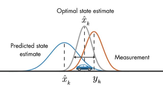
Probabilistic Perspective (Bayesian Estimation)

The filter maintains a Gaussian belief state that gets refined through sequential application of Bayes' rule, where prediction corresponds to Chapman-Kolmogorov propagation and update implements Bayesian conditioning.

$$\begin{array}{rl}& p(x_k|y_{1:k},u_{1:k})\\ =& p(x_k|y_k,y_{1:k-1},u_{1:k})\\ =& \frac{p(y_k|x_k,y_{1:k-1},u_{1:k})\cdot p(x_k|y_{1:k-1},u_{1:k})}{p(y_k|y_{1:k-1},u_{1:k})}\\ =& \eta \cdot \underset{\text{observation model}}{\underbrace{p(y_k|x_k)}}\cdot \underset{\text{prior belief}}{\underbrace{p(x_k|y_{1:k-1},u_{1:k})}}\\ =& \eta \cdot p(y_k|x_k)\cdot \int p(x_k,x_{k-1}|y_{1:k-1},u_{1:k})\mathrm{d}{x}_{k-1}\\ =& \eta \cdot p(y_k|x_k)\cdot \int p(x_k|x_{k-1},y_{1:k-1},u_{1:k})\cdot p(x_{k-1}|y_{1:k-1},u_{1:k})\mathrm{d}{x}_{k-1}\\ =& \eta \cdot p(y_k|x_k)\cdot \int \underset{\text{motion model}}{\underbrace{p(x_k|x_{k-1},u_k)}}\cdot \underset{\text{previous belief}}{\underbrace{p(x_{k-1}|y_{1:k-1},u_{1:k-1})}}\mathrm{d}{x}_{k-1}\\ =& \eta \cdot \mathcal{N}(y_k;H_k{x}_k,R_k)\cdot \int \mathcal{N}(x_k;A{x}_{k-1}+B{u}_k,Q_k)\cdot \mathcal{N}(x_{k-1};{\hat{x}}_{k-1},{\hat{P}}_{k-1})\mathrm{d}{x}_{k-1}\\ =& \eta \cdot \mathcal{N}(y_k;H_k{x}_k,R_k)\cdot \mathcal{N}(x_k;{\hat{x}}_{k|k-1},{\hat{P}}_{k|k-1})\\ \propto & \mathcal{N}(x_k;{\hat{x}}_k,{\hat{P}}_k)\end{array}$$

Applying Bayesian Rule and Markov Assumptions to $p(x_k|y_{1:k},u_{1:k})$, then the time update and the measurement update becomes very explicit.

Optimization Perspective (MAP Estimation)

The Kalman Filter solves a weighted least-squares problem where the optimal state estimate minimizes a cost function balancing prediction fidelity against measurement consistency, with covariance matrices acting as natural weighting matrices.

By Bayesian Rule, we know that

$$p(x_k|y_{1:k},u_{1:k})\propto \underset{\text{measurement}}{\underbrace{p(y_k|x_k)}}\cdot \underset{\text{prior}}{\underbrace{p(x_k|y_{1:k-1},u_{1:k})}}$$

To maximize the posterior probability, it is equivalent to minimizing its negative logarithmic posterior.

$$-\ln p(x_k|y_{1:k},u_{1:k})=-\ln p(y_k|x_k)-\ln p(x_k|y_{1:k-1},u_{1:k})+C$$

Applying Gaussian probability distribution

$$J_{x_k}=\frac{1}{2}||z_k-C{x}_k|{|}_{R_k^{-1}}^2+\frac{1}{2}||x_k-{\hat{x}}_{k|k-1}|{|}_{{\hat{P}}_{k|k-1}}^2+C$$$${\hat{x}}_{k|k-1}=\arg \underset{x_k}{min}(||x_k-{\hat{x}}_{k|k-1}|{|}_{{\hat{P}}_{k|k-1}}^2+|z_k-C{x}_k|{|}_{R_k^{-1}}^2)$$

Prior is given by

$$\begin{array}{rl}{\hat{x}}_{k|k-1}& =\mathbb{E}[x_k|y_{1:k-1},u_{1:k}]\\ {\hat{P}}_{k|k-1}& =\text{Cov}(x_k|y_{1:k-1},u_{1:k})\end{array}$$